In my previous post, I employed a rather crude and non-parametric approach to see if I could predict the direction of stock returns using the function runs.test(). Lets go a step further and try modelling this with a parametric econometric approach. The company that I choose for the study is INFOSYS (NSE code INFY). Lets start by eyeballing the plot of the stock prices of INFY for the past one year.
## Set the working directory using setwd() ##
# Reading the relevant file.
infy <- read.csv("01-10-2010-TO-01-10-2011INFYEQN.csv")
# Plotting the past one year's closing price of INFY
plot(as.Date(infy$Date, "%d-%b-%y"), infy$Close.Price, xlab= "Dates", ylab= "Adjusted closing price", type='l', col='red', main="Adjusted closing price of INFOSYS for past 1 year")
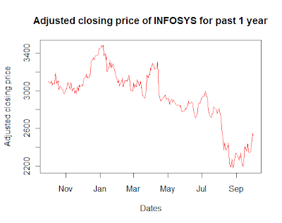
Eyeballing the above plot suggests that the series is NOT second order stationary. Meaning that the first two moments, of the distribution from which the data is drawn, changes with time. For a stationary series, the mean doesn't changes with time and the co-variance with any "k" lag is independent of "t" and it just a function of "k". But we see that both the conditions are violated above.
Let me attempt to explain the idea stationary in simple English language. For a moment suppose that you were to stand at time T = t and look at the value of the series, then look at the neighbors values to the left and right of "t", if by doing this exercise you can make out the value of "t" that you are standing at then it is possibly a non-stationary series. On the other hand if you were placed at time T = t in any stationary series, by doing the above exercise you would not be able to figure out the value of "t". (This definition came up during a discussion with Utkarsh some time ago).
A rule of thumb in any time series modelling is that we work with only stationary time series. If the series exhibits any non-stationarity, we have to remove that before we can employ any empirical analysis. In the above series the non-stationarity can be removed by using the returns instead of actual stock prices. (analogous to First differencing) .
## Calculating the returns of stock prices
infy_ret <- 100*diff(log(infy[,2]))
## Plotting the returns
plot(as.Date(infy$Date[-1], "%d-%b-%y"), infy_ret, xlab= "Dates", ylab= "Returns percentage(%)", type='l', col='red', main="Daily returns of INFOSYS for past 1 year")

We see that in the above plot the mean is fixed at 0 and the fluctuations are around that mean, that doesn't change with time. Now that we have taken care of the non-stationarity lets proceed on our task.
First we will plot the auto-correlation of the returns with the previous lags and see if there is any significant correlation that the returns have with the previous values.
## Plotting the ACF of INFY returns for the past one years
acf(infy_ret, main = "ACF of INFOSYS returns for past one year")

The blue dotted line is the 95% confidence interval. We can see that there is the 4th and the 7th lag significant in the ACF plot (there is one significant at 19th lag too but I choose to ignore that). Now lets see what I get if I regress the value of returns on the lagged values till lag 8th.
## Regressing the returns till the 7th lag
summary(lm(infy_ret[8:length(infy_ret)] ~ infy_ret[8:length(infy_ret) - 1] + infy_ret[8:length(infy_ret) - 2]+ infy_ret[8:length(infy_ret) - 3] + infy_ret[8:length(infy_ret) - 4] + infy_ret[8:length(infy_ret) - 5] + infy_ret[8:length(infy_ret) - 6] +infy_ret[8:length(infy_ret) - 7] ))## This is a simple OLS regression of the "inty_ret" starting from the 8th observation. I have started from the 8th observation to ensure that the number of obs. are same in the dependents and independent variables.
Output:
Coefficients:
Only the coefficient of the 4th lag is statistically significant, and the Adjusted R-squared is a small 0.05998 (i.e ~ 6% of the explanation is provided by the above regression).
In the previous post we had reached the conclusion that the returns series is completely random (using runs.test()). But here we have fit in a model that provides ~ 6% of the explanation, the important question that needs to be addressed now is that the can we use this model to predict the stock returns (and make some money using a trading strategy that employs the above regression).
The model suggests that there is a statistically significant explanation that is being offered by the 4th lag in the above regression, but is this explanation economically significant? Now is when the economic intuition comes into play. The given sample data for the stock prices of INFY for the paste one year has confessed that the 4 days ago stock price provides a statistically significant explanation of today's stock prices. But a major point, perhaps the most important, that we are missing in the above model is the transaction costs or market micro-structures.
Meaning that a statistically significant 4th lag does not mean that the explanation offered is economically significant too. To check if the relation is economically significant, we will have to adjust the prices for transaction costs and then do the regression and see if we get a similar result. Efficient market hypothesis that this statistical significant will disappear once you account for these transaction costs (impact cost or cost of trading). It seems to be intuitive too, because if we look at the ACF plotted above the auto-correlations are not significantly different from 0 and once we account for the transaction costs the 95% band will also broaden.
## Set the working directory using setwd() ##
# Reading the relevant file.
infy <- read.csv("01-10-2010-TO-01-10-2011INFYEQN.csv")
# Plotting the past one year's closing price of INFY
plot(as.Date(infy$Date, "%d-%b-%y"), infy$Close.Price, xlab= "Dates", ylab= "Adjusted closing price", type='l', col='red', main="Adjusted closing price of INFOSYS for past 1 year")

Eyeballing the above plot suggests that the series is NOT second order stationary. Meaning that the first two moments, of the distribution from which the data is drawn, changes with time. For a stationary series, the mean doesn't changes with time and the co-variance with any "k" lag is independent of "t" and it just a function of "k". But we see that both the conditions are violated above.
Let me attempt to explain the idea stationary in simple English language. For a moment suppose that you were to stand at time T = t and look at the value of the series, then look at the neighbors values to the left and right of "t", if by doing this exercise you can make out the value of "t" that you are standing at then it is possibly a non-stationary series. On the other hand if you were placed at time T = t in any stationary series, by doing the above exercise you would not be able to figure out the value of "t". (This definition came up during a discussion with Utkarsh some time ago).
A rule of thumb in any time series modelling is that we work with only stationary time series. If the series exhibits any non-stationarity, we have to remove that before we can employ any empirical analysis. In the above series the non-stationarity can be removed by using the returns instead of actual stock prices. (analogous to First differencing) .
## Calculating the returns of stock prices
infy_ret <- 100*diff(log(infy[,2]))
## Plotting the returns
plot(as.Date(infy$Date[-1], "%d-%b-%y"), infy_ret, xlab= "Dates", ylab= "Returns percentage(%)", type='l', col='red', main="Daily returns of INFOSYS for past 1 year")

We see that in the above plot the mean is fixed at 0 and the fluctuations are around that mean, that doesn't change with time. Now that we have taken care of the non-stationarity lets proceed on our task.
First we will plot the auto-correlation of the returns with the previous lags and see if there is any significant correlation that the returns have with the previous values.
## Plotting the ACF of INFY returns for the past one years
acf(infy_ret, main = "ACF of INFOSYS returns for past one year")

The blue dotted line is the 95% confidence interval. We can see that there is the 4th and the 7th lag significant in the ACF plot (there is one significant at 19th lag too but I choose to ignore that). Now lets see what I get if I regress the value of returns on the lagged values till lag 8th.
## Regressing the returns till the 7th lag
summary(lm(infy_ret[8:length(infy_ret)] ~ infy_ret[8:length(infy_ret) - 1] + infy_ret[8:length(infy_ret) - 2]+ infy_ret[8:length(infy_ret) - 3] + infy_ret[8:length(infy_ret) - 4] + infy_ret[8:length(infy_ret) - 5] + infy_ret[8:length(infy_ret) - 6] +infy_ret[8:length(infy_ret) - 7] ))## This is a simple OLS regression of the "inty_ret" starting from the 8th observation. I have started from the 8th observation to ensure that the number of obs. are same in the dependents and independent variables.
Output:
Coefficients:
                                 Estimate Std. Error t value Pr(>|t|)
(Intercept)                      -0.09316    0.11321  -0.823  0.41140
infy_ret[8:length(infy_ret) - 1]  0.08158    0.06479   1.259  0.20920
infy_ret[8:length(infy_ret) - 2] -0.04017    0.06537  -0.614  0.53950
infy_ret[8:length(infy_ret) - 3] -0.10049    0.06528  -1.539  0.12504
infy_ret[8:length(infy_ret) - 4]  0.20153    0.06457   3.121  0.00203 **
infy_ret[8:length(infy_ret) - 5] -0.08566    0.06568  -1.304  0.19344
infy_ret[8:length(infy_ret) - 6] -0.06849    0.06584  -1.040  0.29928
infy_ret[8:length(infy_ret) - 7] -0.12395    0.06621  -1.872  0.06241 .
---
Signif. codes:  0 ‘***’ 0.001 ‘**’ 0.01 ‘*’ 0.05 ‘.’ 0.1 ‘ ’ 1

Multiple R-squared: 0.08717, Adjusted R-squared: 0.05998
Only the coefficient of the 4th lag is statistically significant, and the Adjusted R-squared is a small 0.05998 (i.e ~ 6% of the explanation is provided by the above regression).
In the previous post we had reached the conclusion that the returns series is completely random (using runs.test()). But here we have fit in a model that provides ~ 6% of the explanation, the important question that needs to be addressed now is that the can we use this model to predict the stock returns (and make some money using a trading strategy that employs the above regression).
The model suggests that there is a statistically significant explanation that is being offered by the 4th lag in the above regression, but is this explanation economically significant? Now is when the economic intuition comes into play. The given sample data for the stock prices of INFY for the paste one year has confessed that the 4 days ago stock price provides a statistically significant explanation of today's stock prices. But a major point, perhaps the most important, that we are missing in the above model is the transaction costs or market micro-structures.
Meaning that a statistically significant 4th lag does not mean that the explanation offered is economically significant too. To check if the relation is economically significant, we will have to adjust the prices for transaction costs and then do the regression and see if we get a similar result. Efficient market hypothesis that this statistical significant will disappear once you account for these transaction costs (impact cost or cost of trading). It seems to be intuitive too, because if we look at the ACF plotted above the auto-correlations are not significantly different from 0 and once we account for the transaction costs the 95% band will also broaden.
So the lesson is that a simple regression of current returns on the lagged returns (auto regressive model in time series parlance) might not be a reliable trading strategy :-)
P.S. In case anyone wishes to replicate the exercise the data can be obtained from here.

